Triangulation Lookup Table as a Simple Solution for Time-to-Arrival Multilateration
Working with my buddy Brad we found out we were both contemplating the same problem, each having arrived there through different means (my own as a contemplation for isolating point sources for sound in a noisy environment and automatically canceling the ambience with 3 or 4 microphones instead of hundreds). Simply put, we needed to, based on nothing more than multiple audio channels, find out where a sound was coming from within a grid (assuming the the audio channels are being produced by microphones placed in 4 corners).
As we dissected the problem, we found 3 things:
- This is a fun real-world problem to chew on.
- It is far more complex than it appears on the surface.
- There are very good, well-documented solutions to this problem – if you’re a mathematician (there’s lots of free math out there, but not a good public library of implemented multilateration code).
Seeing as how neither Brad nor I are super big on the mathematics (that’s what computers are for, after all), we decided to flip the problem on its head: instead of trying to find the intersection of hyperboles in three dimensions, why not pre-calculate the anticipated signal fingerprints in terms of sets of time-to-arrival differences for each of the sensor locations, and then do a nearest-neighbor calculation in the resulting lookup table? I’ll go through the problem deconstruction and solution in steps so it’s easier to see what we were trying to do.
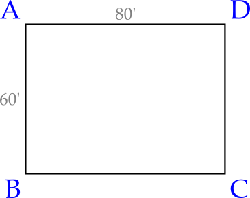
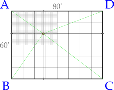
Imagine a grid, say 80′ by 60′, with one microphone placed in each of the 4 corners A, B, C, and D:
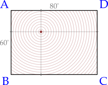
An “audio event” (say, a sneeze, a clap, a code word, etc.) takes place at a random location within our grid, and the sound begins to propagate outward in all directions (rebounding echoes are not shown here, since they will always reach any sensore after the initial sound wave – obstruction based on the direction of the emitter [e.g., which way our sneezer is facing] is also not directly factored in, but has less of a dampening effect than you might think – at least for sounds above a certain threshold):
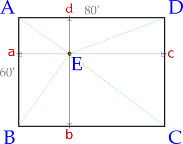
It’s easy to see the distance from this randomly selected point to all 4 corners just by counting rings, but ring counting is not available to us, so we instead use some basic functions and turn the whole thing into right triangles and hypotenuses, so that we may infer from the hypotenuse what the relative lengths are of the other sides and thus our (x,y) coordinates:
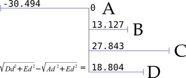
We have now assigned our audio event the label E and assigned the intermediate intersections a, b, c, and d (instead of sticking with just x and y because I want to be able to describe intermediate line segments without confusion). There’s just one problem with this approach – we don’t actually know the distance of any line segment to E! We do know what some of them are relative to each other, though as illustrated in the following figure – but since we don’t know exactly when the sound was first emitted we have to start our counting when the sound reaches the first microphone:
Our signal starts at -30.494ms relative to A, but we don’t know that – all we know is that it was the first to receive the signal, as the closest microphone, and can then count upward from there to the other sensors – which I’ve listed here in sensor order, rather than detection order. Going counter-clockwise like this means that, from the first microphone starting at 0, we will always be seeing adjacent-opposite-adjacent corners (with opposite always the highest number as well).
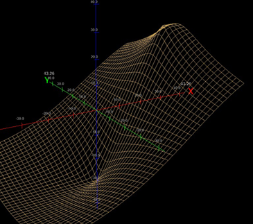
The equation shown next to D is the crux of all this: the value that we record there relative to A is the same as the DE hypotenuse minus the AE hypotenuse as drawn in Figure 3. This relative value is consistent, and follows a predictable curve (shown here from the perspective of time-of-arrival offset at D):
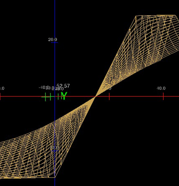
Switching to a dark background here to make the plot more visible. The peak and valley are the bounds of the grid – the fixed distance of the microphones. The slope directly between those 2 points is far more linear, and actual crosses 0 (since AE is going to be greater than DE 50% of the time, some of the values on this graph will be negative, unless you wrap it in an abs function) at the same x on all values, with 0 representing the moment at which the signal will reach both points simultaneously – right smack in the middle. It’s easier to see this from the side:
So we know there’s a plot function for creating this kind of value, but inverting that into something like f(80,18.804) = ED is a little trickier than I’m up for. This is where multilateration comes in, looking for the intersect of 2 such measurements, which requires a lot of propagation along vectors to identify. This is where Brad and I started to cheat: if we can compute what the signal difference would be relative to all 4 microphones for any x,y point on the grid, why not do that in advance at an acceptable resolution, and then look for nearest-neighbor matches to do a look-up instead? With the microphone nearest the event always registering 0 (the starting point for counting), you’re left with the difference of the hypotenuses for the 3 other corners BE, CE, and DE, which produce a nice x,y,z set of coordinates that can be measured against each other.
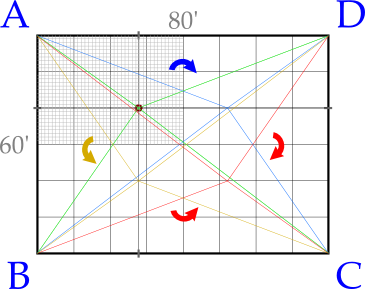
In order to optimize our solution, we take our cue from the fact that the nearest microphone always being 0 means that we only have to compute one quadrant of our grid, which can then be rotated (technically we would only need to calculate half of the quadrant, split diagonally, but computers like grids instead of triangles so we stuck with that):
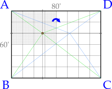
By setting our mapping interval to 1′ that’s the resolution we’re limited to, but for this application is sufficient. The equivalency of the grid is shown through the following 2 figures demonstrating rotation of the event plot:
Given the equivalency, we only need to calculate the relative values to its peers from the perspective of a single designated 0 corner, and then compensate for rotation (which includes swapping adjacent corners if we’ve rotated an interval of 90° [but not 180°]). The real value of this optimization is that it cuts the amount of data we need to scan by 75%. Another optimization is that, when searching row by row through each column, once the coordinate set we’ve evaluated begins to increase in distance the search within that column can be aborted. The most optimal solution would probably be an octree implementation for the coordinate scanning, which would significantly cut the number of neighbor comparisons that need to be made especially on larger data sets – but we didn’t bother going that far.
One problem with this approach though, is that when you don’t have an equal number of units on both x and y axes, you lose a little precision when doing 90º interval rotation by a factor of x:y. Not terrible, but between the trade-offs in resolution and precision, this solution, simple though it may be, is not for everyone.
Crude though the code may be (I hacked it together in Perl initially, then put it into PHP as a lingua franca for Brad – all while commuting on the train) I offer it for your inspection and deconstruction. Bon apetit!
Latest Comments:
Comments are closed for this post.

thank you very much for this informative thread !
Hi Paul,
I’ve been continuing my work on this project and will probably be doing some field testing after the first of the year. I’ll be renting a small community / reception center and setting up all the audio equipment to run the tests.
I have an idea to test your problem/solution subsequent to my tests. All we will need is a few dozen friends to help out.
Are you still interested?
Sure thing!
So the rest of the world knows as well, there are also very good papers and commercial solutions available on this too: